Structure and lineaments

Can gold-bearing structures be read from satellite alone?

More confidently than any other free layer in this package — with one firm caveat.

Orogenic gold in Archaean greenstone belts is structurally controlled. The metal sits in and along shear zones, second- and third-order faults, fold hinges, and lithological contacts that acted as fluid plumbing during deformation. Those structures leave a topographic and a radar-texture signature that a free 30 m DEM and free Sentinel-1 SAR resolve below the scale of the 1:100 000 Geological Survey sheet, which is exactly the gap inside a 300 ha claim.

Satellite-alone gives you a defensible map of candidate structures: linear valleys, aligned drainage, breaks-in-slope, fold-shaped ridge curvature, and radar lineaments. What it does not give you is which of those structures is mineralized. A lineament is a candidate to walk and check against strike/dip readings. It is never a confirmed fault, and certainly never a confirmed gold-bearing fault.

Structure is the highest-signal, lowest-ambiguity free layer in this package. A topographic lineament has far fewer plausible non-geological explanations than a SWIR clay ratio does. Vegetation, laterite, and soil moisture wreck spectral indices in a tropical belt; they barely touch a DEM. SAR sees through cloud and, to a degree, through canopy.

Why structure matters for orogenic gold

Orogenic (lode, mesothermal) gold in the Zimbabwe Craton's Mberengwa/Belingwe greenstone belt is emplaced late in the deformation history, when metamorphic fluids migrate along the most permeable pathways available. Those pathways are structures:

Second- and third-order structures — subsidiary shears, faults, and fractures branching off the belt-scale first-order shear. This is the scale that matters inside a claim and the scale the regional map misses. Dilational jogs and bends on these host the ore shoots.
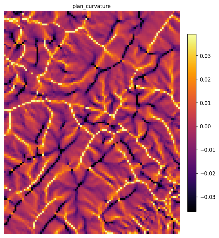
Fold hinges and closures — antiformal closures concentrate fluid; plan and profile curvature flags them from a DEM.
Lithological contacts — the rheological contrast at ultramafic/mafic or BIF contacts localizes strain and hosts listwaenite-style alteration. Contacts often express as a break-in-slope or a drainage line.
Structural intersections — where two trends cross is a classic high-grade target. Lineament intersections carry more weight than lineament length.

The practical exploration heuristic: map the structures, find the second-order splays and the intersections near a favourable lithology, then walk them. Free DEM and SAR let a zero-budget holder do the first two steps from a laptop.

DEM-derived structure

Source and coverage

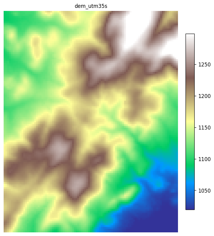
The AOI straddles the E029/E030 one-degree tile boundary at longitude 30.0, so both tiles are fetched from Copernicus GLO-30, reprojected from EPSG:4326 to UTM 35S (EPSG:32735) at 30 m, and mosaicked into a 123 x 97 pixel grid. Elevation ranges from 1006 m to 1341 m across the claim.

import folia

# fetch both tiles (AOI crosses the E029/E030 boundary at lon 30.0)
dem = folia.fetch(
    dataset="@esa/copernicus-dem/glo-30",
    aoi="research/mineral-prospecting/aoi.geojson",
    crs="EPSG:32735",   # reproject to UTM 35S before derivatives
    resolution=30,
)

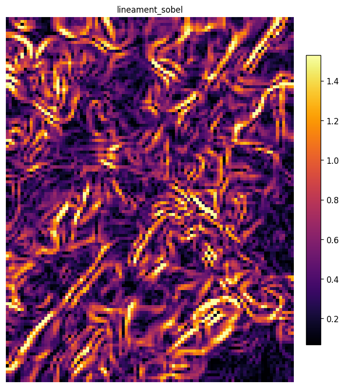
Copernicus GLO-30 DEM mosaicked and reprojected to UTM 35S, showing 1006–1341 m elevation range across the claim — Copernicus GLO-30 DEM, UTM 35S, 30 m. Two tiles mosaicked across the lon 30.0 boundary. Elevation 1006–1341 m.

Multi-azimuth hillshade

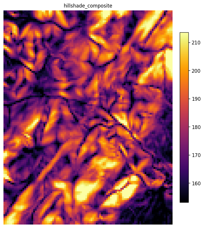
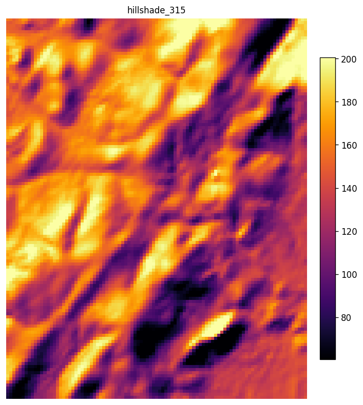
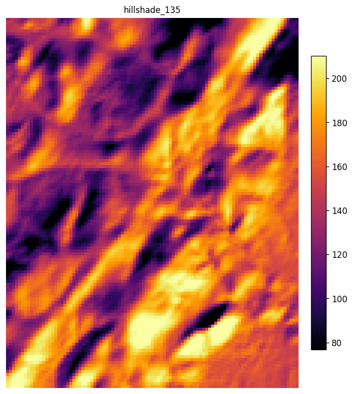
A single hillshade illuminates structures perpendicular to the sun direction and is nearly blind to structures parallel to it. The GIS default of 315 degrees (northwest) systematically under-detects NW-SE structures, which in many cratons is a principal ore-controlling trend.

The fix is multi-azimuth illumination: render hillshades from four azimuths (315, 45, 135, 225 degrees, two orthogonal pairs), then combine them so every structural orientation is lit by at least one sun. The edge-strike rose for this AOI shows a dominant NW-SE trend at 135-150 degrees, a pattern the default single-azimuth hillshade systematically under-detects.

# multi-azimuth hillshade from dem_structure.py
azimuths = [315, 45, 135, 225]
hillshades = [compute_hillshade(dem, azimuth=az, altitude=35) for az in azimuths]
composite = np.max(np.stack(hillshades), axis=0)   # max-lit composite

Source: research/mineral-prospecting/structure-lineaments/dem_structure.py

Multi-azimuth hillshade composite (max of 315, 45, 135, 225 degree illuminations) — Multi-azimuth hillshade composite. All structural orientations are illuminated; the dominant NW-SE trend emerges clearly.

Single-azimuth hillshade, 315 degrees (northwest sun) — 315 degrees (NW sun, the GIS default). NW-SE structures are under-detected.

Single-azimuth hillshade, 135 degrees (southeast sun) — 135 degrees (SE sun). Illuminates the NW-SE trend the default misses.

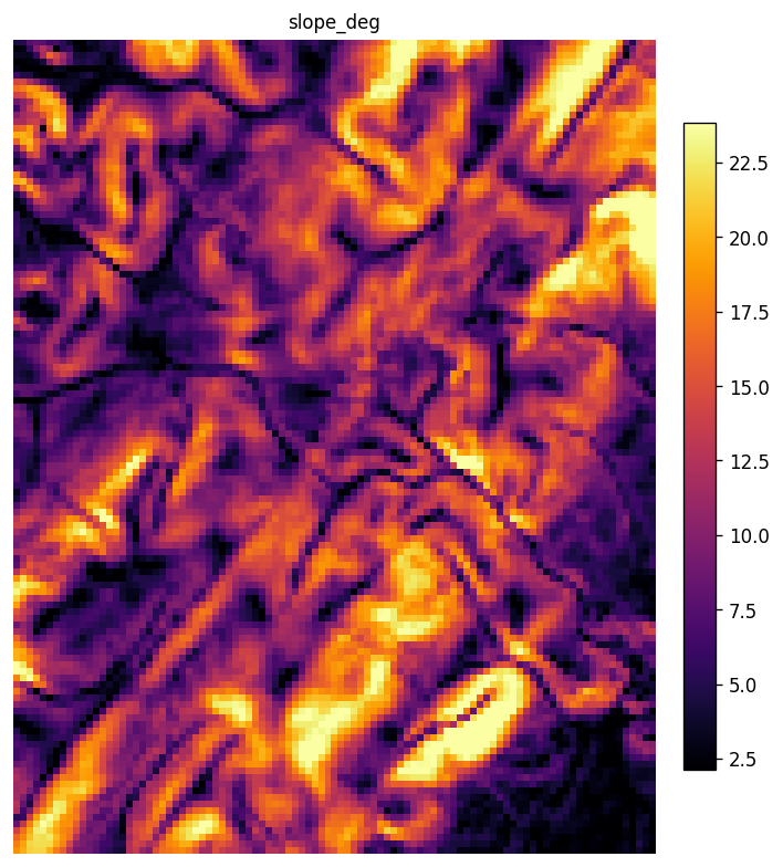
Slope and curvature

Faults and contacts often coincide with linear breaks-in-slope. Fold closures appear as curved arcs of high plan curvature. Profile curvature flags scarp edges and fold-limb-to-hinge transitions.

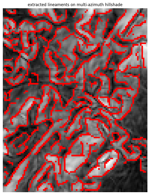
Slope in degrees, derived from the 30 m DEM in UTM 35S — Slope (degrees). Linear steepness transitions trace candidate contacts and fault scarps.

Plan curvature (curvature across the slope direction) — Plan curvature. Fold closures and curved ridgelines appear as arched high-curvature features.

Lineament extraction

Lineaments are extracted by applying a Sobel gradient-magnitude operator to the multi-azimuth hillshade composite, then converting the edge map to vectorised segments. Density is computed as total lineament length per unit area, producing a heatmap of structural complexity. The method is the open-source equivalent of the PCI Geomatica LINE algorithm (Canny/Sobel edge detection, threshold, thin, link) used widely in the mineral-exploration literature.

Sobel gradient-magnitude edge map on the multi-azimuth composite — Sobel edge map on the composite hillshade. Each bright pixel is a candidate structural edge.

Lineament density heatmap: total lineament length per unit area — Lineament density. High-density zones are structurally complex ground and the primary walk targets.

Extracted lineaments overlaid on the composite hillshade. NW-SE and NE-SW trends are both visible; intersections between them are the highest-priority targets.

Drainage as a structural proxy

Rivers exploit weakness: straight stream segments, abrupt right-angle bends, aligned valley reaches, and trellis/rectangular drainage patterns are textbook fault and fracture indicators. A first-order channel that runs straight for a kilometre is following something.

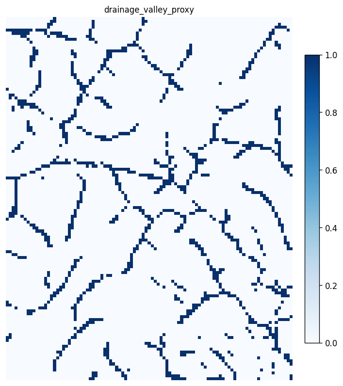
Drainage and valley proxy derived from flow accumulation and curvature — Drainage and valley proxy. Straight or aligned reaches that co-locate with lineament-density highs are reinforced candidates.

Anthropogenic false positives are the dominant confound. Roads, tracks, field edges, terraces, and fence-line erosion all make straight topographic lines. Cross-checking every candidate against optical imagery before calling it structural is mandatory.

SAR-derived structure (Sentinel-1)

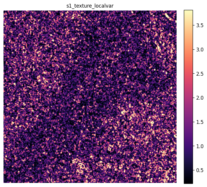
SAR adds an independent structural view with three properties that matter in this belt: it is cloud-proof and day/night capable; its side-looking geometry produces a built-in shaded-relief analog where slopes facing the radar appear bright; and the spatial texture of backscatter separates rough/blocky terrain (rock outcrop, scree along a scarp) from smooth terrain (soil, cultivated ground).

The data used here are Sentinel-1 RTC ascending orbit, 2026-06-21, already in UTM 35S at 10 m. No reprojection is needed.

s1 = folia.fetch(
    dataset="@esa/sentinel-1/rtc",
    aoi="research/mineral-prospecting/aoi.geojson",
    bands=["vv", "vh"],
    date="2026-06-01/2026-06-21",
    crs="EPSG:32735",   # already native; confirmed by inspection
)

Source: research/mineral-prospecting/structure-lineaments/sar_texture.py

Sentinel-1 VV backscatter in dB, Lee speckle-filtered — Sentinel-1 VV (dB), Lee speckle-filtered. Bright returns indicate rough or steep slopes facing the radar.

Sentinel-1 VH backscatter in dB, Lee speckle-filtered — Sentinel-1 VH (dB), Lee speckle-filtered. VH depolarization is sensitive to volume scatterers and surface roughness.

Local variance texture derived from Sentinel-1 VV — Local-variance texture. Linear texture contrasts trace contacts and fault scarps independently of backscatter intensity.

SAR-derived lineaments overlaid on the VV backscatter image — SAR-derived lineaments overlaid on VV. Compare with the DEM lineament map: agreement between the two is the strongest indicator of a real structural feature.

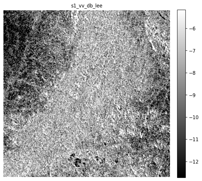
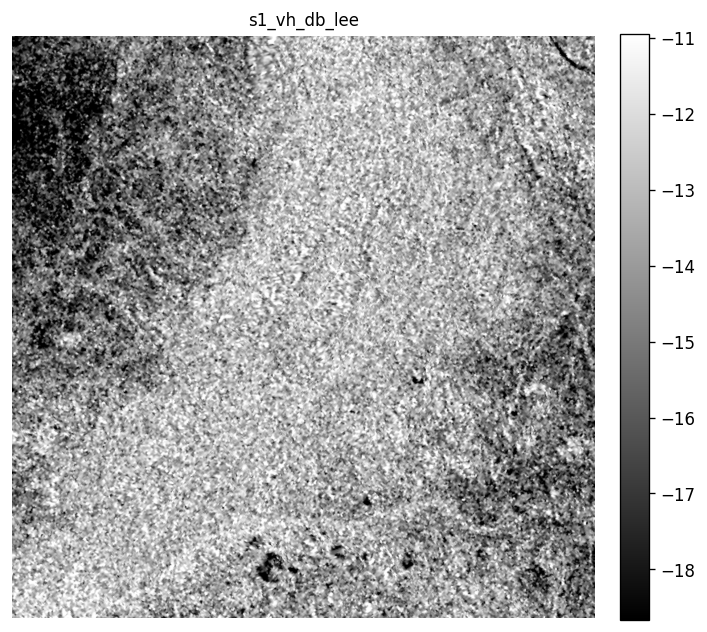
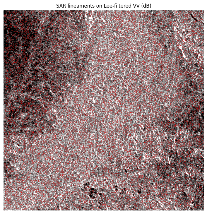
Look-direction bias

SAR has a fixed look direction per orbit pass. Structures parallel to the look direction are foreshortened or invisible; structures perpendicular are enhanced. This is the direct analogue of the hillshade sun-azimuth problem. The mitigation is to combine ascending and descending passes (different look azimuths). This arm uses one scene to demonstrate the method; combining orbit directions is the next production step.

NISAR L-band: when it arrives

C-band (5.6 cm wavelength) backscatter is dominated by the canopy and the top of the vegetation/soil layer. Under closed tropical canopy, Sentinel-1 images the vegetation, not the rock beneath it. L-band (~24 cm, as on NISAR and ALOS-2 PALSAR) penetrates vegetation substantially better and interacts with the ground, trunks, and large branches, giving a structural read the C-band misses.

A coverage probe against the NISAR GCOV beta catalog (NISAR_L2_GCOV_BETA_V1_1, window 2025-10 to 2026-06) returned 0 granules over this AOI. The same search returns 20 beta granules globally, so this is a genuine coverage gap, not a probe failure. Once commissioning coverage reaches this latitude (-20 S), L-band will be the upgrade that sees structure under canopy.

Source: research/mineral-prospecting/structure-lineaments/nisar_coverage_check.py

ALOS PALSAR-2 mosaics offer free L-band coverage now for areas NISAR has not yet reached. They are a practical interim option for sub-canopy structural mapping and a natural next step once the C-band lineament map is validated against field observations.

How to use these outputs

Open the lineament-density heatmap and the multi-azimuth composite side by side. Density highs are structurally complex ground.
Note the dominant trends. The edge-strike rose shows a NW-SE principal at 135-150 degrees; compare this to the belt's known structural grain on the Geological Survey sheet.
Find intersections of two trends near a favourable lithology. These are the top-ranked walk targets.
Overlay the drainage proxy. Straight or aligned channel reaches that co-locate with a lineament-density high reinforce it.
Compare DEM and SAR lineament maps. Features that appear in both are more likely to be structural rather than anthropogenic.
Cross every candidate against the holder's strike/dip readings (in-situ structure.template.csv). A lineament whose azimuth matches a measured shear or fault strike is a calibrated candidate. One that does not match is either a different feature or a structure not yet logged.
Discard anything that is obviously a road or field edge in optical imagery.

Outputs are candidates to field-check, not faults. Nothing here says gold.

Limitations

Layer	Limitation
DEM 30 m	Resolves only tens-of-metres topographic expression. Sub-tile fractures with no relief are invisible.
Anthropogenic false positives	Roads, tracks, field edges, terraces. The dominant DEM-lineament confound. Cross-check optical.
C-band canopy ceiling	Sentinel-1 under closed canopy images vegetation, not rock.
Single SAR scene / single orbit	One ascending scene; no descending pass to mitigate look-direction bias.
No mineralization signal	Structure narrows where to walk. The rock must be sampled to determine ore control.
Uncalibrated without in-situ data	The in-situ structural template is the calibration step; without it, all candidates are equal weight.

The conversion from "lineament" to "ore control" is a field and sample job. This page produces the where-to-walk map. The in-situ structural log (research/mineral-prospecting/in-situ/) is where it gets calibrated against measured strike, dip, and sample results.