Iron oxide and gossans

Can red iron-oxide zones (gossans) be picked out from free Sentinel-2 and Landsat, and with which bands?

Short answer: yes, partially, and as a prioritization layer, not a detector. Ferric iron (Fe³⁺) has a strong, diagnostic reflectance signature that free Sentinel-2 and Landsat both capture. But in a tropical greenstone belt the same signature comes from lateritic soil and weathered mafic bedrock, which are everywhere. The index alone cannot separate a true sulphide gossan from ordinary red dirt. It tells you where the surface is iron-stained. Mapped geological contacts and ground samples are what turn that into a gossan hypothesis.

The spectral basis

Iron oxides and oxyhydroxides — hematite, goethite, limonite, jarosite, the minerals that make a gossan red-brown — owe their colour to Fe³⁺ electronic transitions. The practical consequences for broadband satellites:

Strong absorption in the blue (~0.45 µm) and a charge-transfer drop into the near-UV. Blue reflectance is low over iron-oxide surfaces.
Rising reflectance through red (~0.65 µm) into the near-infrared. There is also a broad Fe³⁺ crystal-field absorption near 0.85–0.90 µm (the ferric edge) and a deeper Fe²⁺ feature near 1.0 µm.
The contrast red-high/blue-low is the whole reason a simple red-to-blue ratio works as an iron-oxide index. A ratio also divides out topographic shading, since both bands dim together on a shadowed slope.

Hydroxyl/clay (Al-OH, Mg-OH) and carbonate features sit further out at 2.2–2.35 µm and are the subject of the companion alteration mapping arm. This arm is about iron specifically.

Recommended band ratios

Sentinel-2 (10–20 m, free, 5-day revisit)

Index	Formula	What it keys on
Iron-oxide ratio	B04 / B02 (red / blue)	Red-high, blue-low signals ferric staining. S2 B04 ≈ 665 nm, B02 ≈ 490 nm, both 10 m. The workhorse.
Ferric-iron SWIR	B11 / B08	Ferric absorption rising into SWIR vs the NIR shoulder. B11 ≈ 1610 nm (20 m), B08 ≈ 842 nm (10 m); resampled to a common grid. Catches more weathered/oxidized surfaces than red/blue alone.
Crosta iron PC	Directed PCA over B02, B04, B08, B11	The principal component whose B04 and B02 loadings have opposite signs. Suppresses albedo and vegetation that contaminate a simple ratio; isolates the ferric contrast direction.

A secondary S2 ratio in the literature is B11/B12 (1610/2190 nm) for broad ferric/ferrous discrimination. Van der Werff and van der Meer (2016) show S2's SWIR sampling is coarse but usable for relative iron mapping. The three above are the core; B11/B12 is a one-line extension.

Landsat Collection-2 Level-2 (30 m, free) — cross-check

Index	Formula	Equivalent
Iron-oxide ratio	band4 / band2 (red / blue)	The classic Landsat ferric ratio (Sabins 1999), exactly the S2 B04/B02 at coarser 30 m.

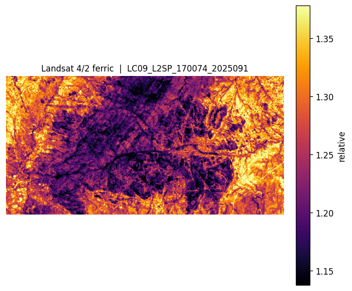
The Landsat 4/2 ratio is used only as an independent-sensor sanity check: if the same patches light up at 30 m on a different platform, the S2 signal is less likely to be a single-scene artifact.

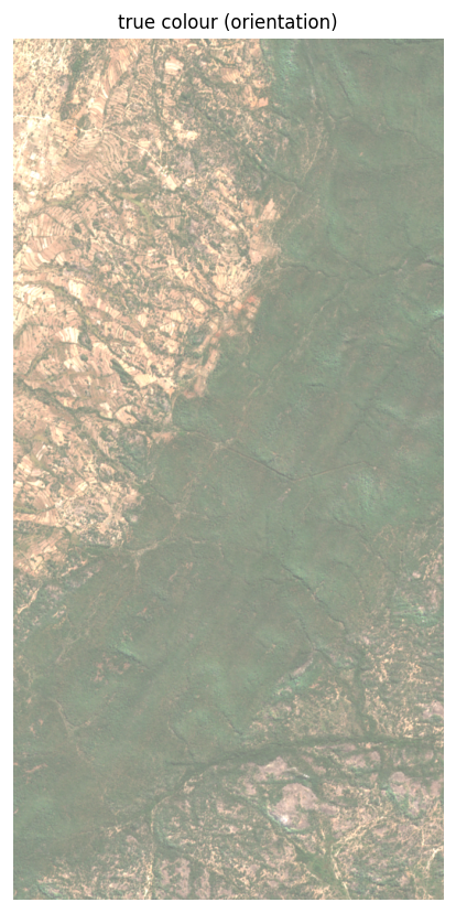
Bands to fetch for this arm. Sentinel-2: B02, B03, B04, B08, B11, B12, SCL (B03 is only for the true-colour orientation image). Landsat: red, blue.

The scene

The analysis uses a single Sentinel-2A Level-2A scene: T35KRT, acquired 2025-06-21, 0% cloud cover (MGRS tile covering the Mberengwa/Belingwe greenstone belt, Zimbabwe). Dry-season acquisition is intentional: phenology is at its lowest biomass, maximising exposed-soil fractions for a mineralogy-sensitive window.

Sentinel-2 true colour composite of the study AOI, 2025-06-21 — Sentinel-2 true colour (B04-B03-B02), 2025-06-21. Dense tropical canopy (dark green) covers the majority of the frame; exposed laterite and bare soil appear as red-brown tones.

Index outputs

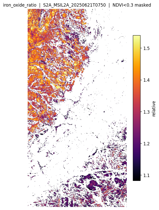
Iron-oxide ratio (B04 / B02)

The ratio ranges approximately 1.08–1.54 across valid (unmasked) pixels in this scene. Values above 1 are expected everywhere since red always exceeds blue; the relative brightness is the signal.

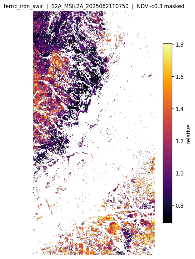
Sentinel-2 B04/B02 iron-oxide ratio, stretched 2–98th percentile — B04/B02 ferric ratio, 2–98th percentile stretch. Brighter zones indicate stronger iron-oxide staining. Masked pixels (cloud, shadow, dense canopy) are shown as no-data.

Ferric iron SWIR (B11 / B08)

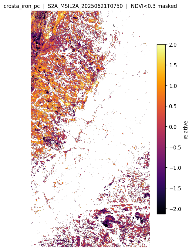
Sentinel-2 B11/B08 ferric SWIR ratio — B11/B08 ratio. Sensitive to more weathered and oxidized surfaces than the visible ratio alone. The two indices are complementary rather than redundant.

Crosta directed PCA iron component

The Crosta technique selects the PCA component whose loadings match the ferric spectral contrast: high B04, low B02, with B08 and B11 adding sensitivity to the ferric edge and SWIR shoulder. On this scene the chosen component has loadings approximately B02 ≈ −0.88 and B04 ≈ +0.47, confirming it tracks the ferric contrast direction. The script prints the full loading vector so you can verify it on any new scene.

Landsat cross-check (band4 / band2)

Landsat Collection-2 band4/band2 iron-oxide ratio at 30 m — Landsat C2-L2 band4/band2 at 30 m. Same spatial clusters as the S2 ratio, confirming the signal is not a single-sensor artefact. Resolution is coarser but coverage and archive depth are greater.

What the outputs show (with caveats)

High-index pixels form spatially coherent clusters rather than speckle — a good sign that the indices are tracking real surface variation. However, much of that variation is almost certainly laterite and weathered greenstone, exactly as the spectral physics predicts.

~72% of the AOI is canopy-masked. The dense tropical canopy removes roughly three quarters of all pixels from analysis. The indices speak only for the ~28% of exposed or sparse-canopy ground. Any gossan beneath continuous canopy is invisible to this approach.

Laterite is the dominant false positive. Deep tropical weathering produces red hematite/goethite-rich lateritic soil across large areas. It is spectrally near-identical to a gossan cap. Weathered greenstone-belt basalts and komatiites similarly weather to iron-rich surfaces. The background in this terrain is iron-stained, not the anomaly.

Broadband indices cannot distinguish hematite from goethite from jarosite. That distinction, which can hint at gossan vs laterite, requires hyperspectral or narrow SWIR sensors (EMIT, EnMAP, PRISMA, ASTER). This arm is the cheap, always-available first pass. The alteration mapping arm covers the hyperspectral ceiling.

How to use the output honestly

Three mitigations keep the map useful despite the false-positive problem:

SCL masking removes cloud, shadow, cirrus, saturated, and no-data pixels so they do not generate fake anomalies.
NDVI masking (NDVI > 0.30) removes dense canopy; the index only reports on bare or sparse ground where iron staining is actually observable.
Relative, per-scene, percentile-stretched output. No absolute "this is a gossan" threshold is claimed. Brighter means look here first, within this scene.

The real discriminator is external: overlay high-index zones on the geological survey lithology and structure sheet. A bright patch on a mapped contact, fault, or shear zone is a far stronger gossan hypothesis than an equally bright patch in the middle of a laterite plateau.

When ground samples are available, the calibration hook in the script (currently dormant) measures whether each index meaningfully elevates at known gossan points versus background. A separability score greater than 1σ means the index is worth trusting for prioritization at this site; a score near zero means you should lean on structure and contacts instead.

Literature

Sabins (1999), Remote sensing for mineral exploration, Ore Geology Reviews. Canonical source for the broadband ratio toolkit, including the red/blue ferric ratio used here and the caution that ratios are relative anomaly maps requiring field control.
Crosta and Moore (1989); Loughlin (1991). Directed / feature-oriented PCA: select the principal component whose loadings match the target mineral's known spectral contrast. More robust than a raw ratio because it down-weights albedo and vegetation.
Van der Werff and van der Meer (2016), Sentinel-2 for mapping iron absorption feature parameters, Remote Sensing. Establishes that S2's band placement, despite being designed for vegetation, samples the ferric absorption well enough for relative iron-oxide mapping, and quantifies where its coarse SWIR sampling limits mineral specificity relative to hyperspectral sensors.

Recipe

The indices are computed by fetch_and_index.py. The key fetch call and ratio formula:

import folia
import numpy as np

# Fetch S2 L2A bands windowed to the AOI
# Scene: S2A T35KRT, 2025-06-21, 0% cloud
ds = folia.fetch(
    collection="sentinel-2-l2a",
    item="S2A_MSIL2A_20250621T075021_R135_T35KRT_20250621T112615",
    bands=["B02", "B03", "B04", "B08", "B11", "B12", "SCL"],
    aoi=aoi_geom,
    backend="planetary-compute",  # anonymous, no auth required
)

# Scale DN to surface reflectance
refl = {b: ds[b].values * 1e-4 for b in ["B02", "B04", "B08", "B11"]}

# Iron-oxide ratio (Sabins 1999 ferric VNIR)
iron_oxide = refl["B04"] / np.where(refl["B02"] > 0, refl["B02"], np.nan)

# Ferric SWIR
ferric_swir = refl["B11"] / np.where(refl["B08"] > 0, refl["B08"], np.nan)

# Apply vegetation + cloud mask before analysis
valid = (ndvi < 0.30) & scl_valid_mask
iron_oxide = np.where(valid, iron_oxide, np.nan)

Full recipe at research/mineral-prospecting/iron-oxide-gossan/fetch_and_index.py

One-line summary for any briefing: This map shows where the ground is iron-stained on a cloud-free dry-season scene. It will also highlight laterite and weathered greenstone. Treat bright zones that coincide with mapped contacts and structures as walk-first targets, not as confirmed gossans, and never as gold detections.