Alteration mapping
Research question 2a: Can alteration zones be read from satellite alone, without a ground-truthed spectral library?
Short answer: Yes for a relative anomaly, no for a mineral identity — and the gap between those two is the whole story.
1. Assemblage first: orogenic, not epithermal
Most "alteration mapping with satellite" tutorials are built around epithermal gold systems, whose advanced-argillic halos carry alunite, kaolinite, and dickite — minerals with sharp, separable Al-OH absorptions near 2.16–2.20 µm that ASTER maps beautifully. That is the canonical story. It is the wrong story for a greenstone belt.
Orogenic (mesothermal / lode) gold forms deeper, in metamorphosed greenstone, along shears and faults. Its alteration assemblage is:
| Halo zone | Minerals | Diagnostic absorption | Sensor that can see it |
|---|---|---|---|
| Phyllic / sericitic (proximal) | sericite, muscovite, illite | Al-OH ~2200 nm | ASTER SWIR b5–b7; HSI; S2 only coarsely |
| Propylitic / carbonate (distal, listwaenite) | chlorite, epidote, calcite / dolomite / ankerite | Mg-OH / carbonate ~2300–2350 nm | ASTER SWIR b7–b9; HSI; not S2 |
| Silicification | quartz | TIR emissivity minimum ~9 µm (no SWIR feature) | ASTER TIR (post-2008 OK); HSI: no |
| Gossan / sulphide (oxidised) | Fe-oxides | Fe³⁺ VNIR | S2 / Landsat — see iron-oxide arm |
Two consequences for this analysis: the carbonate / Mg-OH 2300–2350 nm feature is at least as important as the Al-OH feature (carbonate alteration and listwaenite are classic orogenic-gold vectors), and silica has no shortwave feature at all — it shows only as a TIR emissivity low, which ASTER's surviving TIR detector can read.
Getting the assemblage wrong is the most common way these analyses go silently wrong.
2. Why band ratios need no calibrated library
A spectral library is needed when you want to match a pixel's full spectrum to a named mineral — shape-fitting against reference curves. That is identity, and it requires calibrated, continuum-removed reflectance compared to known endmembers.
A band ratio asks a smaller, library-free question: within this one scene, is band X relatively brighter or darker than band Y at this pixel?
- It compares the scene to itself, so absolute radiometric calibration to a library is unnecessary — the ratio is dimensionless.
- It divides out first-order topographic shading and illumination (both bands dim together on a shaded slope), which matters in steep greenstone terrain.
- A mineral with an absorption in band Y and a shoulder in band X produces a high X/Y ratio relative to the rest of the scene, flagging an anomaly without ever naming the mineral.
Ratios give you a relative alteration anomaly map for free, with no library and no ground truth. What they cannot give you is which mineral — that ceiling is set by how many, and how narrow, the sensor's SWIR bands are.
3. Sentinel-2: a coarse proxy and its hard limit
S2 was designed for vegetation and land cover, not geology. In the SWIR it has only two bands, both at 20 m:
B11  ~1610 nm  (1565–1655)
B12  ~2190 nm  (2100–2280)
The standard relative clay/hydroxyl ratio is B11 / B12 — the two-SWIR-band analogue of the Landsat TM 5/7 clay ratio. It works, but note what B12's window swallows:
Implemented indices
| Index | Formula | Keys on | Honest read |
|---|---|---|---|
| Clay / hydroxyl | B11 / B12 | relative SWIR hydroxyl anomaly | coarse, undifferentiated; clay-rich laterite lights up like real alteration |
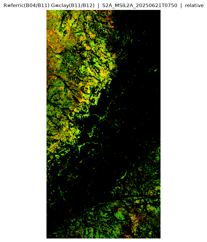
| Ferric–clay composite | B04 / B11 plotted against B11/B12 | two relative axes side by side | lets the holder eyeball "iron-ish vs clay-ish" without fusing into one ambiguous score |
Bands fetched: B04, B08, B11, B12, SCL. B04 and B08 build the NDVI vegetation mask; SCL removes cloud, shadow, cirrus, saturated, and no-data pixels (classes 0, 1, 3, 8, 9, 10).
# research/mineral-prospecting/alteration-mapping/s2_alteration.py
import folia

# fetch S2 L2A bands over the claim AOI
ds = folia.fetch(
    "@esa/sentinel-2/l2a",
    aoi=AOI_GEOJSON,
    bands=["B04", "B08", "B11", "B12", "SCL"],
    date_range=("2023-01-01", "2024-12-31"),
    cloud_cover_max=20,
)

# relative clay/hydroxyl ratio (library-free, self-referential)
clay_hydroxyl = ds["B11"] / ds["B12"]

# vegetation mask (suppress false positives over dense canopy)
ndvi = (ds["B08"] - ds["B04"]) / (ds["B08"] + ds["B04"])
clay_hydroxyl = clay_hydroxyl.where(ndvi < 0.4)
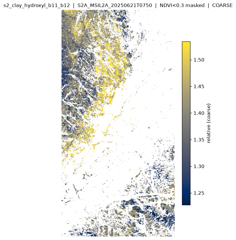
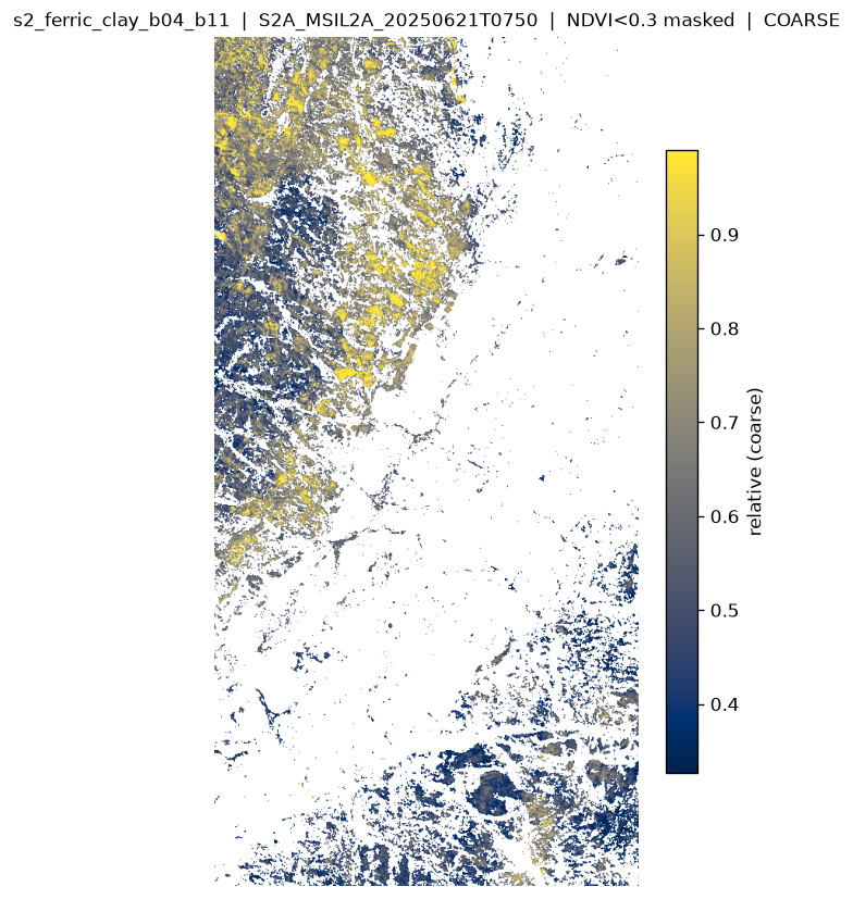
The S2 answer to Q2a: yes, you get a free, always-available, library-free screening layer for clay/hydroxyl alteration. It is coarse and ambiguous — a "look here first," never a mineral map. This is the floor; ASTER and imaging spectroscopy are the ceiling.
4. ASTER: the right multispectral tool (pre-2008 SWIR only)
ASTER's six SWIR bands at 30 m were designed to straddle exactly the orogenic alteration features S2 blurs together:
ASTER SWIR band centres (µm):
  b4 1.65   b5 2.165   b6 2.205   b7 2.26   b8 2.33   b9 2.395
                        └─Al-OH──┘           └──Mg-OH / carbonate──┘
Al-OH / phyllic index (proximal sericite halo)
Rowan and Mars (2003) phyllic ratio: b5 / b6 — high where the b6 trough marks the Al-OH absorption at 2.205 µm. Variants include b7 / b6 and (b5 + b7) / b6.
Carbonate / Mg-OH / chlorite index (distal halo, listwaenite)
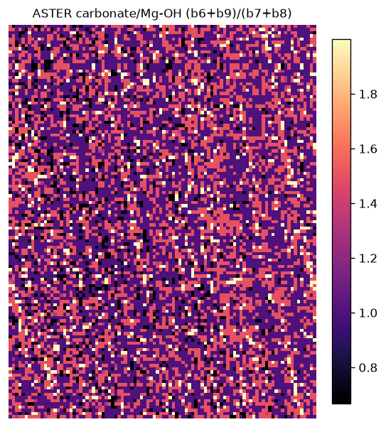
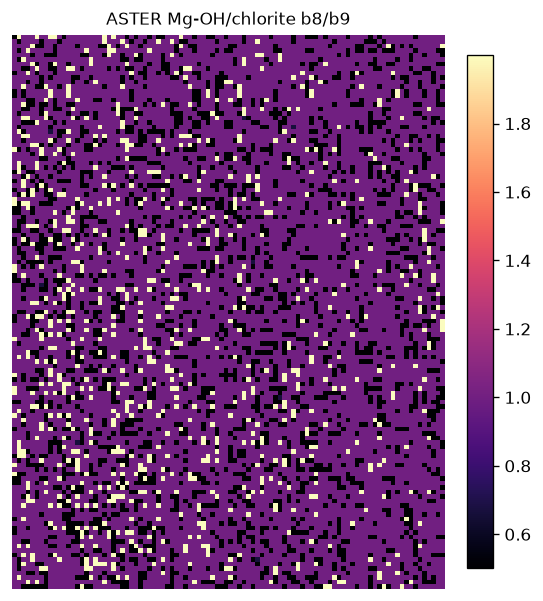
Rowan and Mars (2003) carbonate index: (b6 + b9) / (b7 + b8) — high over the 2.3–2.35 µm carbonate/Mg-OH absorption straddled by b8. A related index, b8 / b9, targets Mg-OH and chlorite more specifically.
These are relative ratios, not mineral maps — the same logic as §2.
# research/mineral-prospecting/alteration-mapping/aster_alteration.py
import numpy as np
import rasterio
from rasterio.windows import from_bounds
import folia

# folia: discovery and URL signing (ASTER SWIR is one 6-band COG, not per-band)
# folia.fetch() returns only band 1 of a multiband COG, so we sign then read
# directly via rasterio — see implementation note below
items = folia.catalog.items_for_aoi(
    "@nasa/aster/l1t",
    aoi=AOI_GEOJSON,
    date_range=("2000-01-01", "2008-01-01"),
)
swir_url = folia.catalog._sign_url(items[0].assets["SWIR"].href)

with rasterio.open(swir_url) as src:
    window = from_bounds(*AOI_BOUNDS_UTM, transform=src.transform)
    # bands 1–6 of the SWIR COG = ASTER b4–b9 in order
    arr = src.read(window=window).astype(float)
    arr[arr == 0] = np.nan          # mask DN=0 no-data

b4, b5, b6, b7, b8, b9 = arr[0], arr[1], arr[2], arr[3], arr[4], arr[5]

aloh      = b5 / b6                      # Al-OH / phyllic (sericite)
carbonate = (b6 + b9) / (b7 + b8)       # carbonate / Mg-OH
mgoh      = b8 / b9                      # Mg-OH / chlorite
folia.fetch() returns only band 1 of a multiband COG. ASTER ships its SWIR data as a single 6-band COG, so the script uses folia for discovery and URL signing, then performs the windowed multiband read directly via rasterio. This is a genuine reader gap for multiband COGs, consistent with the known Python/TS COG-reader divergence in the platform. A ticket to handle multiband reads natively is warranted if multiband COGs become common.
ASTER's ceiling: even six SWIR bands discriminate mineral groups (Al-OH vs Mg-OH/carbonate), not species (muscovite vs illite vs phengite). For an arbitrary claim, a usable pre-2008 SWIR scene is roughly a coin-flip; this claim is fortunate.
5. Pre-2008 ASTER coverage of this claim
aster_alteration.py queries @nasa/aster/l1t on the Microsoft Planetary Computer, whose ASTER subset spans approximately 2000–2006 — entirely within the usable SWIR window. Five pre-2008 scenes intersect the AOI, all carrying the SWIR asset. The 2005-11-13 scene was selected and processed.
| Date | Scene ID |
|---|---|
| 2000-08-22 | AST_L1T_00308222000082657_20150411060450 |
| 2001-06-27 | AST_L1T_00306272001204859_20170807204458 |
| 2003-01-26 | AST_L1T_00301262003081917_20150426232615 |
| 2003-11-19 | AST_L1T_00311192003081243_20150502022320 |
| 2005-11-13 | AST_L1T_00311132005204014_20170801221104 (used) |
Outputs are relative Al-OH and carbonate/Mg-OH anomaly ratios written to outputs/aster_*.tif and outputs/aster_coverage.json. They are not mineral maps. The right next step is to overlay the Al-OH and carbonate highs on the structure-lineaments layer and the holder's field notes — alteration on a mapped structure is a far stronger vector than alteration in isolation.
6. Imaging spectroscopy: the true ceiling, and EMIT coverage
The honest top of the ladder is imaging spectroscopy: hundreds of contiguous narrow bands that resolve the shape of the 2200 nm and 2300–2350 nm features well enough to identify sericite vs chlorite vs carbonate by spectral-feature fitting.
EMIT (NASA, on the ISS, approximately 285 bands at 7.5 nm, 60 m) images within approximately ±52° latitude. emit_coverage_check.py queries @nasa/emit/l2a-reflectance via the open STAC browse API (no download).
# research/mineral-prospecting/alteration-mapping/emit_coverage_check.py
import folia

items = folia.catalog.search(
    "@nasa/emit/l2a-reflectance",
    aoi=AOI_GEOJSON,
    date_range=("2022-01-01", "2026-12-31"),
)
# prints granule ids, dates, cloud fraction
# writes outputs/emit_coverage.json
# no byte download — EMIT L2A is behind Earthdata Login
Seven EMIT L2A granules intersect the AOI (2024–2026); three are cloud-free:
| Date | Cloud cover | Granule ID |
|---|---|---|
| 2024-02-23 | 0 % | EMIT_L2A_RFL_001_20240223T115131_2405408_006 |
| 2024-03-02 | 4 % | EMIT_L2A_RFL_001_20240302T084202_2406206_006 |
| 2024-05-02 | 0 % | EMIT_L2A_RFL_001_20240502T083431_2412305_056 |
| 2024-11-04 | 0 % | EMIT_L2A_RFL_001_20241104T065732_2430904_013 |
| 2024-11-12 | 100 % | EMIT_L2A_RFL_001_20241112T132436_2431708_041 |
| 2025-01-15 | 83 % | EMIT_L2A_RFL_001_20250115T120359_2501507_030 |
| 2026-03-02 | 100 % | EMIT_L2A_RFL_001_20260302T074345_2606105_019 |
outputs/emit_coverage.json.
PRISMA (ASI) and EnMAP (DLR) would also resolve this assemblage. Both are tasked sensors (you request an acquisition; archives are thin and partly access-gated) and neither exposes an open STAC catalog to probe the way EMIT does. They are named here as the true tool, not a fetchable layer.
7. Literature
- Ninomiya, Y. (2003). "A stabilized vegetation index and several mineralogic indices defined for ASTER VNIR/SWIR/TIR data." IGARSS. Defines the OH-bearing, carbonate, and quartz/silica indices used industry-wide.
- Rowan, L.C. and Mars, J.C. (2003). "Lithologic mapping in the Mountain Pass, California area using ASTER data." Remote Sensing of Environment 84(3): 350–366. The widely cited Al-OH (b5/b6) and carbonate ((b6+b9)/(b7+b8)) ratio recipes.
- Mars, J.C. and Rowan, L.C. (2006). "Regional mapping of phyllic- and argillic-altered rocks in the Zagros magmatic arc, Iran, using Advanced Spaceborne Thermal Emission and Reflection Radiometer (ASTER) data and logical operator algorithms." Geosphere 2(3): 161–186. Combines SWIR ratios into decision-rule alteration maps.
- van der Werff, H. and van der Meer, F. (2016). "Sentinel-2 for mapping iron absorption feature parameters." Remote Sensing 8(12): 1035. Quantifies where S2's coarse SWIR sampling limits mineral specificity vs ASTER and HSI — the basis for §3's ceiling.
8. The honest answer
You can map an alteration anomaly from satellite alone with no spectral library, because band ratios are relative, self-referential contrasts that need no calibrated endmembers. What you cannot do with free Sentinel-2 is identify the alteration mineral: its two coarse SWIR bands fuse the Al-OH (2200 nm) and carbonate/Mg-OH (2300–2350 nm) features into one undifferentiated number. Real mineral discrimination needs more SWIR resolution: ASTER's six SWIR bands (available here on five pre-2008 scenes) separate the Al-OH and carbonate halos into distinct relative indices; and imaging spectroscopy — EMIT, which covers this claim with seven granules, three cloud-free — resolves feature shapes well enough to name minerals via the package's shape-fitting engines.
Across all three sensors, the output is a where-to-walk-first layer to be cross-checked against mapped structures and ground samples. No pixel — S2, ASTER, or EMIT — should be read as "this is sericite." None of them should be read as "this is gold."